Tutorial B: Process the downloaded data¶

heiplanet-data Python package - data processing and visualization of the processed data

---

Authors: Scientific Software Center
Date: October 2025
Version: 1.0

---

Overview¶

This tutorial demonstrates how to process downloaded data files through heiplanet-data. You will learn how to:

1. Specify the settings for heiplanet-data: Work with settings files to store data transformations
2. Data operations: Carry out different data operations such as resampling of the grid
3. Data Visualization: Create plots to verify the processed data

heiplanet-data¶

The heiplanet-data package can help you transform your data in an efficient way, and stores the settings alongside your data to ensure reproducibility. The flow of operations is visualized in this flowchart:

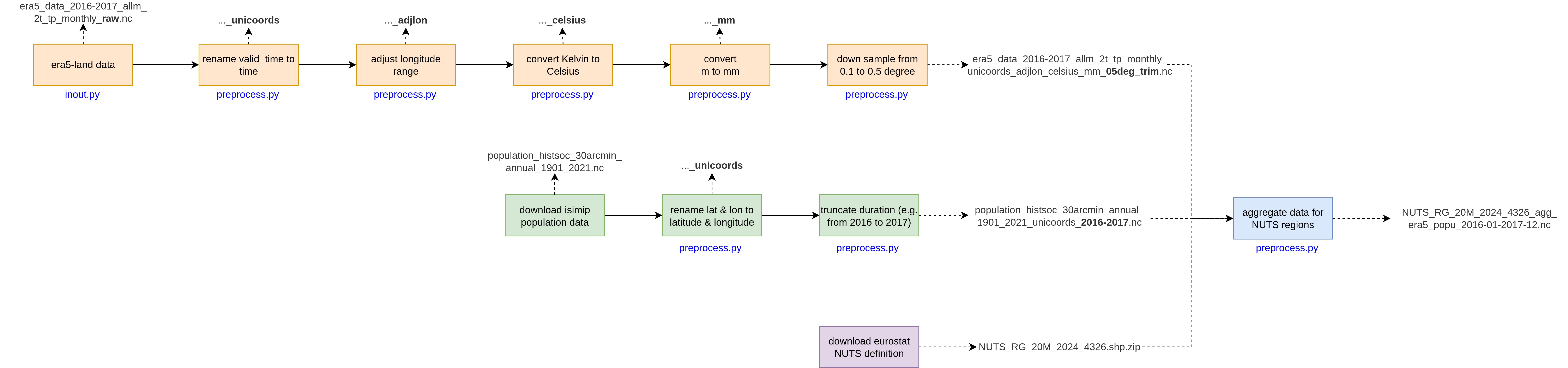
For the different data sources, different operations are carried out:

1. Copernicus data: Here, the columns of the data are renamed from valid_time to time, the longitude is adjusted to lie between -180 and 180 degrees, and the temperature is converted from K to C. Precipitation is converted from m to mm, and the latitude/longitude grid can be resampled to match, for example, the grid resolution of the ISIMIP data.
2. Population data: Here, the columns of the data are renamed from lat to latitude and long to longitude, further, the range of years with data is truncated to a specified range.

We will look at NUTS data and averaging in the next part of the tutorial, tutorial C. For now, let's start by importing the necessary libraries.

In [ ]:

# if running on google colab
# flake8-noqa-cell

if "google.colab" in str(get_ipython()):
    # install packages
    %pip install git+https://github.com/ssciwr/heiplanet-data.git -qqq

# if running on google colab # flake8-noqa-cell if "google.colab" in str(get_ipython()): # install packages %pip install git+https://github.com/ssciwr/heiplanet-data.git -qqq

Since we will be downloading some data on-the-fly using pooch, you also need to have this library installed in your environment (i.e. pip install pooch.)

In [ ]:

from heiplanet_data import preprocess
from pathlib import Path
import json
import time
import pooch
import xarray as xr
from matplotlib import pyplot as plt

from heiplanet_data import preprocess from pathlib import Path import json import time import pooch import xarray as xr from matplotlib import pyplot as plt

In [ ]:

# change to your own data folder, if needed
data_root = Path("data/")
data_folder = data_root / "in"
era5_fname = "era5_data_2016-2017_allm_2t_tp_monthly_raw.nc"
era5_fpath = data_folder / era5_fname
isimip_fname = "population_histsoc_30arcmin_annual_1901_2021.nc"
isimip_fpath = data_folder / isimip_fname

# change to your own data folder, if needed data_root = Path("data/") data_folder = data_root / "in" era5_fname = "era5_data_2016-2017_allm_2t_tp_monthly_raw.nc" era5_fpath = data_folder / era5_fname isimip_fname = "population_histsoc_30arcmin_annual_1901_2021.nc" isimip_fpath = data_folder / isimip_fname

1. Settings specifications¶

We use preprocess module to perform preprocessing steps, using function named preprocess_data_file():

def preprocess_data_file(
    netcdf_file: Path,
    source: Literal["era5", "isimip"] = "era5",
    settings: Path | str = "default",
    new_settings: Dict[str, Any] | None = None,
    unique_tag: str | None = None,
) -> Tuple[xr.Dataset, str]:

Here, netcdf_file defines the path to the input file, while source indicates whether the .nc file is downloaded from ERA5-Land or ISIMIP as these two sources have different preprocessing steps. This is relevant if you are loading default settings. If you are loading a custom settings file for custom data, as we will see later, you should specify the source as era5.

The preprocessing steps are determined using a dictionary (JSON file), providied through the settings parameter. This parameter can either be set to a file path or to the string "default". If a file path is given, the settings will be loaded from that file; if loading fails, the default settings for the corresponding source era5 or isimip will be used instead. If "default" is specified, the default settings of the relevant source are loaded directly.

If only certain fields of the default settings need to be updated, these fields and their values can be supplied as a dictionary via the new_settings parameter.

The final settings used for preprocessing are saved to a file in the same directory as the preprocessed .nc file. This output directory is defined in the provided settings file. The unique_tag is appended to both the settings file and the resulting .nc file to link them together. By default, this is a combination of host name and date.

The settings keys for the data (pre-)processing are defined as follows - you can consult this table when you adjust the settings for your specific data:

keyword	type and default value	description
output_dir	string, default: "data/processed"	Directory where processed data will be saved.
adjust_longitude	boolean, default: true	Whether to adjust longitude values to the range [-180, 180].
adjust_longitude_vname	string, default: "longitude"	Variable name of the longitude values to adjust.
adjust_longitude_fname	string, default: "adjlon"	Suffix of file names after adjusting longitude values.
convert_kelvin_to_celsius	boolean, default: true	Whether to convert temperature values from Kelvin to Celsius.
convert_kelvin_to_celsius_vname	string, default: "t2m"	Variable name of the temperature values to convert.
convert_kelvin_to_celsius_fname	string, default: "celsius"	Suffix of file names after converting temperature values to Celsius.
convert_m_to_mm_precipitation	boolean, default: true	Whether to convert precipitation values from meters to millimeters.
convert_m_to_mm_precipitation_vname	string, default: "tp"	Variable name of the precipitation values to convert.
convert_m_to_mm_precipitation_fname	string, default: "mm"	Suffix of file names after converting precipitation values to millimeters.
resample_grid	boolean, default: true	Whether to resample the grid to a specified resolution.
resample_grid_vname	array of strings, default: ["latitude", "longitude"]	Variable names of the latitude and longitude values for resampling.
resample_degree	number, default: 0.5	Value of the target grid resolution in degrees.
resample_grid_fname	string, default: "deg_trim"	Suffix of file names after resampling the grid.
truncate_date	boolean, default: true	Whether to truncate the time series from a specified date.
truncate_date_from	string, default: "2016-01-01"	Date in YYYY-MM-DD to truncate the time series from.
truncate_date_to	string, default: "2017-12-31"	Date in YYYY-MM-DD to truncate the time series to.
truncate_date_vname	string, default: "time"	Variable name of the time values to truncate.
unify_coords	boolean, default: true	Whether to unify coordinate names in the data file.
unify_coords_fname	string, default: "unicoords"	Suffix of file names after unifying coordinate names.
uni_coords	object, default: {"lat": "latitude", "lon": "longitude", "valid_time": "time"}	Mapping of variable names to their new names.

The following subsections illustrate how the settings in the preprocessing are applied to ERA5-Land data and ISIMIP data.

2. Data operations¶

Preprocess ERA5-Land data¶

Default settings for .nc files from ERA5-Land are:

{
    "output_dir": "processed",          # Directory for saved processed files
    "adjust_longitude": true,                         # Enable longitude adjustment to [-180, 180] range
    "adjust_longitude_vname": "longitude",            # Variable name for longitude values
    "adjust_longitude_fname": "adjlon",               # File suffix after longitude adjustment
    "convert_kelvin_to_celsius": true,                # Enable temperature conversion from K to °C
    "convert_kelvin_to_celsius_vname": "t2m",         # Variable name for temperature data
    "convert_kelvin_to_celsius_fname": "celsius",     # File suffix after temperature conversion
    "convert_m_to_mm_precipitation": true,            # Enable precipitation conversion from m to mm
    "convert_m_to_mm_precipitation_vname": "tp",      # Variable name for precipitation data
    "convert_m_to_mm_precipitation_fname": "mm",      # File suffix after precipitation conversion
    "resample_grid": true,                            # Enable grid resampling to specified resolution
    "resample_grid_vname": ["latitude", "longitude"], # Variable names for lat/lon coordinates
    "resample_degree": 0.5,                           # Target grid resolution in degrees
    "resample_grid_fname": "deg_trim",                # File suffix after grid resampling
    "unify_coords": true,                             # Enable coordinate name standardization
    "unify_coords_fname": "unicoords",                # File suffix after coordinate unification
    "uni_coords": {                                   # Mapping of old to new coordinate names
        "valid_time": "time"                          # Rename 'valid_time' to 'time'
    }
}

The output directory for all preprocessed files and utilized settings files is set to path "processed". This path is relative to the current file. For .nc files downloaded from ERA5-Land, we need to perform the following preprocessing steps:

• adjust longitude from range $[0..360]$ to $[-180..180]$
• convert temperature values from Kelvin to Celsius
• convert precipitation values from meter to millimeter
• resample the grid from $0.1°$ to $0.5°$
• rename coordinates to a unified name set, i.e. latitude, longitude, and time

We toggle these steps by setting the corresponding field to true or false, e.g. "unify_coords": false disables coordinate renaming.

Fields end with _vname specify which data variables in a .nc file will be used for the corresponding preprocessing step. While fields with _fname define the suffix to add into the file name after the preprocessing step run successfully. For an overview of file name transformation, see flowchart in heiplanet-data section.

Ultimately, the uni_coords dictionary defines the mapping between old and new coordinate names.

In [ ]:

print(f"Preprocessing ERA5-Land data: {era5_fpath}")
t0 = time.time()
preprocessed_dataset, era5_pfname = preprocess.preprocess_data_file(
    netcdf_file=era5_fpath,
    source="era5",
    settings="default",
    new_settings=None,
    unique_tag="tutorial_B",
)
t_preprocess = time.time()
print(f"Preprocessing completed in {t_preprocess - t0:.2f} seconds.")
print(f"Name of preprocessed file: {era5_pfname}")

print(f"Preprocessing ERA5-Land data: {era5_fpath}") t0 = time.time() preprocessed_dataset, era5_pfname = preprocess.preprocess_data_file( netcdf_file=era5_fpath, source="era5", settings="default", new_settings=None, unique_tag="tutorial_B", ) t_preprocess = time.time() print(f"Preprocessing completed in {t_preprocess - t0:.2f} seconds.") print(f"Name of preprocessed file: {era5_pfname}")

Preprocess population data¶

Default settings for .nc files from ISIMIP are:

{
    "output_dir": "processed",    # Directory for saved processed files
    "truncate_date": true,                      # Enable time series truncation to specific date range
    "truncate_date_from": "2016-01-01",         # Start date for data truncation (YYYY-MM-DD format)
    "truncate_date_to": "2017-12-31",           # End date for data truncation (YYYY-MM-DD format)
    "truncate_date_vname": "time",              # Variable name for time dimension
    "unify_coords": true,                       # Enable coordinate name standardization
    "unify_coords_fname": "unicoords",          # File suffix after coordinate unification
    "uni_coords": {                             # Mapping of old to new coordinate names
        "lat": "latitude",                      # Rename 'lat' to 'latitude'
        "lon": "longitude"                      # Rename 'lon' to 'longitude'
    }
}

The resulting files (data and settings) will be saved into output_dir (relative path to the current file). To preprocess .nc files from ISIMIP, we consider these steps:

• truncate data in a specific range, with start and end timepoints included
• unify coordinate names

The naming convention for fields in these settings follows the same pattern described above for ERA5-Land.

In [ ]:

print(f"Preprocessing ISIMIP data: {isimip_fpath}")
t0 = time.time()
preprocessed_popu, isimip_pfname = preprocess.preprocess_data_file(
    netcdf_file=isimip_fpath,
    source="isimip",
    settings="default",
    new_settings=None,
    unique_tag=None,
)
t_popu = time.time()
print(f"Preprocessing ISIMIP data completed in {t_popu - t0:.2f} seconds.")
print(f"Name of preprocessed file: {isimip_pfname}")

print(f"Preprocessing ISIMIP data: {isimip_fpath}") t0 = time.time() preprocessed_popu, isimip_pfname = preprocess.preprocess_data_file( netcdf_file=isimip_fpath, source="isimip", settings="default", new_settings=None, unique_tag=None, ) t_popu = time.time() print(f"Preprocessing ISIMIP data completed in {t_popu - t0:.2f} seconds.") print(f"Name of preprocessed file: {isimip_pfname}")

Process custom data¶

For custom data, there are no default settings. You should specify the source type as era5 when you call the preprocess function, and provide your own custom dictionary with the desired settings. An example is shown here for model predictions, resampling the prediction to a grid of 0.25 degrees resolution from an initial 0.5 degrees resolution.

First we need to download the data. The below cell will fail if you do not have pooch installed in your environment, in which case you need to pip install pooch.

In [ ]:

# Download the custom data
filename = "output_JModel_global.nc"
url = "https://heibox.uni-heidelberg.de/f/ce8cfdab18da414fb259/?dl=1"
filehash = "df6f6062b57608a6a05afe51653b1fa51219190c67c2e34924e4719609ce6182"
try:
    file = pooch.retrieve(
        url=url,
        known_hash=filehash,
        fname=filename,
        path=data_folder,
    )
except Exception as e:
    print(f"Error fetching data: {e}")
    raise RuntimeError(f"Failed to fetch data from {url}") from e
print(f"Data fetched and saved to {file}")

# Download the custom data filename = "output_JModel_global.nc" url = "https://heibox.uni-heidelberg.de/f/ce8cfdab18da414fb259/?dl=1" filehash = "df6f6062b57608a6a05afe51653b1fa51219190c67c2e34924e4719609ce6182" try: file = pooch.retrieve( url=url, known_hash=filehash, fname=filename, path=data_folder, ) except Exception as e: print(f"Error fetching data: {e}") raise RuntimeError(f"Failed to fetch data from {url}") from e print(f"Data fetched and saved to {file}")

In [ ]:

jmodel_fpath = data_folder / "output_JModel_global.nc"
settings_file_path = data_folder / "settings_JModel_global.json"

jmodel_fpath = data_folder / "output_JModel_global.nc" settings_file_path = data_folder / "settings_JModel_global.json"

We are providing a settings_file_path, where we can either deposit a settings file that contains the settings to be used (for example, if you rerun the same processes multiple times), or we can also save the current settings as input to that file. Note that the settings are always also stored with your processed data, so that you can reproduce any processing steps.

For now, we will define the settings in this notebook and store them in settings_file_path:

In [ ]:

settings = {
    "output_dir": "processed",
    "resample_grid": True,  # Enable grid resampling to specified resolution
    "resample_grid_vname": [
        "latitude",
        "longitude",
    ],  # Variable names for lat/lon coordinates
    "resample_degree": 0.25,  # Target grid resolution in degrees
    "resample_grid_fname": "deg_trim",  # File suffix after grid resampling
}
# write the settings to a json file
json.dump(settings, open(settings_file_path, "w"))

settings = { "output_dir": "processed", "resample_grid": True, # Enable grid resampling to specified resolution "resample_grid_vname": [ "latitude", "longitude", ], # Variable names for lat/lon coordinates "resample_degree": 0.25, # Target grid resolution in degrees "resample_grid_fname": "deg_trim", # File suffix after grid resampling } # write the settings to a json file json.dump(settings, open(settings_file_path, "w"))

Now we can preprocess the custom data file, using the settings defined above:

In [ ]:

print(f"Preprocessing JModel output data: {jmodel_fpath}")
t0 = time.time()
preprocessed_jmodel, jmodel_pfname = preprocess.preprocess_data_file(
    netcdf_file=jmodel_fpath,
    source="era5",
    settings=settings_file_path,
    new_settings=None,
    unique_tag=None,
)
t_jmodel = time.time()
print(f"Preprocessing JModel data completed in {t_jmodel - t0:.2f} seconds.")
print(f"Name of preprocessed file: {jmodel_pfname}")

print(f"Preprocessing JModel output data: {jmodel_fpath}") t0 = time.time() preprocessed_jmodel, jmodel_pfname = preprocess.preprocess_data_file( netcdf_file=jmodel_fpath, source="era5", settings=settings_file_path, new_settings=None, unique_tag=None, ) t_jmodel = time.time() print(f"Preprocessing JModel data completed in {t_jmodel - t0:.2f} seconds.") print(f"Name of preprocessed file: {jmodel_pfname}")

Alternatively, you can provide the settings as a dictionary to new_settings, overwriting the era5 default settings on the go.

3. Creating plots of the (pre-)processed data¶

For this, we again use xarray and read the data into xarray datasets.

In [ ]:

era5_ds_processed = xr.open_dataset(Path.cwd() / "processed" / era5_pfname)
isimip_ds_processed = xr.open_dataset(Path.cwd() / "processed" / isimip_pfname)
jmodel_ds_processed = xr.open_dataset(Path.cwd() / "processed" / jmodel_pfname)

# for a comparison, also open the raw ERA5 data
era5_ds_raw = xr.open_dataset(era5_fpath)
isimip_ds_raw = xr.open_dataset(isimip_fpath)
jmodel_ds_raw = xr.open_dataset(jmodel_fpath)

era5_ds_processed = xr.open_dataset(Path.cwd() / "processed" / era5_pfname) isimip_ds_processed = xr.open_dataset(Path.cwd() / "processed" / isimip_pfname) jmodel_ds_processed = xr.open_dataset(Path.cwd() / "processed" / jmodel_pfname) # for a comparison, also open the raw ERA5 data era5_ds_raw = xr.open_dataset(era5_fpath) isimip_ds_raw = xr.open_dataset(isimip_fpath) jmodel_ds_raw = xr.open_dataset(jmodel_fpath)

Now we can plot the era5 processed and raw data for selected months.

In [ ]:

# create a plot for raw and processed data next to each other
# plot the cartesian grid data of t2m for 2016-2 and 2016-8

selected_times = [
    "2016-01-01",
    "2016-07-01",
]

# Create figure with subplots for temperature comparison
fig, axes = plt.subplots(2, 2, figsize=(12, 8))
fig.suptitle("ERA5 Temperature Data Comparison: Raw vs Processed", fontsize=16, y=0.94)

# Plot raw data
for i, time_val in enumerate(selected_times):
    raw_data = era5_ds_raw.sel(valid_time=time_val, method="nearest")
    im1 = raw_data.t2m.plot.pcolormesh(
        ax=axes[0, i], cmap="coolwarm", robust=True, add_colorbar=False
    )
    axes[0, i].set_title(f"Raw - {time_val[:7]}", pad=15)

    processed_data = era5_ds_processed.sel(time=time_val, method="nearest")
    im2 = processed_data.t2m.plot.pcolormesh(
        ax=axes[1, i], cmap="coolwarm", robust=True, add_colorbar=False
    )
    axes[1, i].set_title(f"Processed - {time_val[:7]}", pad=15)

# Adjust layout with more spacing
plt.tight_layout(rect=[0, 0.05, 0.98, 0.94])  # Leave space for colorbars on the right
plt.subplots_adjust(hspace=0.4, wspace=0.3)  # Add space between subplots

# Add separate colorbars for each row
cbar1 = fig.colorbar(im1, ax=axes[0, :], orientation="vertical", pad=0.02, shrink=0.8)
cbar1.set_label("Raw Temperature (K)", fontsize=10)

cbar2 = fig.colorbar(im2, ax=axes[1, :], orientation="vertical", pad=0.02, shrink=0.8)
cbar2.set_label("Processed Temperature (°C)", fontsize=10)

plt.show()

# create a plot for raw and processed data next to each other # plot the cartesian grid data of t2m for 2016-2 and 2016-8 selected_times = [ "2016-01-01", "2016-07-01", ] # Create figure with subplots for temperature comparison fig, axes = plt.subplots(2, 2, figsize=(12, 8)) fig.suptitle("ERA5 Temperature Data Comparison: Raw vs Processed", fontsize=16, y=0.94) # Plot raw data for i, time_val in enumerate(selected_times): raw_data = era5_ds_raw.sel(valid_time=time_val, method="nearest") im1 = raw_data.t2m.plot.pcolormesh( ax=axes[0, i], cmap="coolwarm", robust=True, add_colorbar=False ) axes[0, i].set_title(f"Raw - {time_val[:7]}", pad=15) processed_data = era5_ds_processed.sel(time=time_val, method="nearest") im2 = processed_data.t2m.plot.pcolormesh( ax=axes[1, i], cmap="coolwarm", robust=True, add_colorbar=False ) axes[1, i].set_title(f"Processed - {time_val[:7]}", pad=15) # Adjust layout with more spacing plt.tight_layout(rect=[0, 0.05, 0.98, 0.94]) # Leave space for colorbars on the right plt.subplots_adjust(hspace=0.4, wspace=0.3) # Add space between subplots # Add separate colorbars for each row cbar1 = fig.colorbar(im1, ax=axes[0, :], orientation="vertical", pad=0.02, shrink=0.8) cbar1.set_label("Raw Temperature (K)", fontsize=10) cbar2 = fig.colorbar(im2, ax=axes[1, :], orientation="vertical", pad=0.02, shrink=0.8) cbar2.set_label("Processed Temperature (°C)", fontsize=10) plt.show()

Note that due to the different scale between K and C, the shading of the plots is slightly different.

In [ ]:

# the same for the precipitation
fig, axes = plt.subplots(2, 2, figsize=(12, 8))
fig.suptitle(
    "ERA5 Precipitation Data Comparison: Raw vs Processed", fontsize=16, y=0.94
)

# Plot raw data
for i, time_val in enumerate(selected_times):
    raw_data = era5_ds_raw.sel(valid_time=time_val, method="nearest")
    im1 = raw_data.tp.plot.pcolormesh(
        ax=axes[0, i], cmap="Blues", robust=True, add_colorbar=False
    )
    axes[0, i].set_title(f"Raw - {time_val[:7]}", pad=15)

    processed_data = era5_ds_processed.sel(time=time_val, method="nearest")
    im2 = processed_data.tp.plot.pcolormesh(
        ax=axes[1, i], cmap="Blues", robust=True, add_colorbar=False
    )
    axes[1, i].set_title(f"Processed - {time_val[:7]}", pad=15)

# Adjust layout with more spacing
plt.tight_layout(rect=[0, 0.05, 0.98, 0.94])  # Leave space for colorbars on the right
plt.subplots_adjust(hspace=0.4, wspace=0.3)  # Add space between subplots

# Add separate colorbars for each row
cbar1 = fig.colorbar(im1, ax=axes[0, :], orientation="vertical", pad=0.02, shrink=0.8)
cbar1.set_label("Raw precipitation (m)", fontsize=10)

cbar2 = fig.colorbar(im2, ax=axes[1, :], orientation="vertical", pad=0.02, shrink=0.8)
cbar2.set_label("Processed precipitation (mm)", fontsize=10)

plt.show()

# the same for the precipitation fig, axes = plt.subplots(2, 2, figsize=(12, 8)) fig.suptitle( "ERA5 Precipitation Data Comparison: Raw vs Processed", fontsize=16, y=0.94 ) # Plot raw data for i, time_val in enumerate(selected_times): raw_data = era5_ds_raw.sel(valid_time=time_val, method="nearest") im1 = raw_data.tp.plot.pcolormesh( ax=axes[0, i], cmap="Blues", robust=True, add_colorbar=False ) axes[0, i].set_title(f"Raw - {time_val[:7]}", pad=15) processed_data = era5_ds_processed.sel(time=time_val, method="nearest") im2 = processed_data.tp.plot.pcolormesh( ax=axes[1, i], cmap="Blues", robust=True, add_colorbar=False ) axes[1, i].set_title(f"Processed - {time_val[:7]}", pad=15) # Adjust layout with more spacing plt.tight_layout(rect=[0, 0.05, 0.98, 0.94]) # Leave space for colorbars on the right plt.subplots_adjust(hspace=0.4, wspace=0.3) # Add space between subplots # Add separate colorbars for each row cbar1 = fig.colorbar(im1, ax=axes[0, :], orientation="vertical", pad=0.02, shrink=0.8) cbar1.set_label("Raw precipitation (m)", fontsize=10) cbar2 = fig.colorbar(im2, ax=axes[1, :], orientation="vertical", pad=0.02, shrink=0.8) cbar2.set_label("Processed precipitation (mm)", fontsize=10) plt.show()

In [ ]:

# the same for the population
selected_times = [
    "2016-01-01",
    "2017-01-01",
]

fig, axes = plt.subplots(2, 2, figsize=(12, 8))
fig.suptitle("Population Data Comparison: Raw vs Processed", fontsize=16, y=0.94)

# Plot raw data
for i, time_val in enumerate(selected_times):
    raw_data = isimip_ds_raw.sel(time=time_val, method="nearest")
    im1 = raw_data["total-population"].plot.pcolormesh(
        ax=axes[0, i], cmap="viridis", robust=True, add_colorbar=False
    )
    axes[0, i].set_title(f"Raw - {time_val[:7]}", pad=15)

    processed_data = isimip_ds_processed.sel(time=time_val, method="nearest")
    im2 = processed_data["total-population"].plot.pcolormesh(
        ax=axes[1, i], cmap="viridis", robust=True, add_colorbar=False
    )
    axes[1, i].set_title(f"Processed - {time_val[:7]}", pad=15)

# Adjust layout with more spacing
plt.tight_layout(rect=[0, 0.05, 0.98, 0.94])  # Leave space for colorbars on the right
plt.subplots_adjust(hspace=0.4, wspace=0.3)  # Add space between subplots

# Add separate colorbars for each row
cbar1 = fig.colorbar(im1, ax=axes[0, :], orientation="vertical", pad=0.02, shrink=0.8)
cbar1.set_label("Total population", fontsize=10)

cbar2 = fig.colorbar(im2, ax=axes[1, :], orientation="vertical", pad=0.02, shrink=0.8)
cbar2.set_label("Total population", fontsize=10)

plt.show()

# the same for the population selected_times = [ "2016-01-01", "2017-01-01", ] fig, axes = plt.subplots(2, 2, figsize=(12, 8)) fig.suptitle("Population Data Comparison: Raw vs Processed", fontsize=16, y=0.94) # Plot raw data for i, time_val in enumerate(selected_times): raw_data = isimip_ds_raw.sel(time=time_val, method="nearest") im1 = raw_data["total-population"].plot.pcolormesh( ax=axes[0, i], cmap="viridis", robust=True, add_colorbar=False ) axes[0, i].set_title(f"Raw - {time_val[:7]}", pad=15) processed_data = isimip_ds_processed.sel(time=time_val, method="nearest") im2 = processed_data["total-population"].plot.pcolormesh( ax=axes[1, i], cmap="viridis", robust=True, add_colorbar=False ) axes[1, i].set_title(f"Processed - {time_val[:7]}", pad=15) # Adjust layout with more spacing plt.tight_layout(rect=[0, 0.05, 0.98, 0.94]) # Leave space for colorbars on the right plt.subplots_adjust(hspace=0.4, wspace=0.3) # Add space between subplots # Add separate colorbars for each row cbar1 = fig.colorbar(im1, ax=axes[0, :], orientation="vertical", pad=0.02, shrink=0.8) cbar1.set_label("Total population", fontsize=10) cbar2 = fig.colorbar(im2, ax=axes[1, :], orientation="vertical", pad=0.02, shrink=0.8) cbar2.set_label("Total population", fontsize=10) plt.show()

And as well for the data from the model output. Here, we have changed the grid resolution (in this case, upsampled), but in a more general case this would be downsampled from a higher to a lower resolution, to preserve accuracy.

In [ ]:

selected_times = [
    "2016-01-01",
    "2016-07-01",
]

# Create figure with subplots for model comparison
fig, axes = plt.subplots(2, 2, figsize=(12, 8))
fig.suptitle("Jmodel Data Comparison: Raw vs Processed", fontsize=16, y=0.94)

# Plot raw data
for i, time_val in enumerate(selected_times):
    raw_data = jmodel_ds_raw.sel(time=time_val, method="nearest")
    im1 = raw_data.R0.plot.pcolormesh(
        ax=axes[0, i], cmap="coolwarm", robust=True, add_colorbar=False
    )
    axes[0, i].set_title(f"Raw - {time_val[:7]}", pad=15)

    processed_data = jmodel_ds_processed.sel(time=time_val, method="nearest")
    im2 = processed_data.R0.plot.pcolormesh(
        ax=axes[1, i], cmap="coolwarm", robust=True, add_colorbar=False
    )
    axes[1, i].set_title(f"Processed - {time_val[:7]}", pad=15)

# Adjust layout with more spacing
plt.tight_layout(rect=[0, 0.05, 0.98, 0.94])  # Leave space for colorbars on the right
plt.subplots_adjust(hspace=0.4, wspace=0.3)  # Add space between subplots

# Add separate colorbars for each row
cbar1 = fig.colorbar(im1, ax=axes[0, :], orientation="vertical", pad=0.02, shrink=0.8)
cbar1.set_label("Raw Temperature (K)", fontsize=10)

cbar2 = fig.colorbar(im2, ax=axes[1, :], orientation="vertical", pad=0.02, shrink=0.8)
cbar2.set_label("Processed Temperature (°C)", fontsize=10)

plt.show()

selected_times = [ "2016-01-01", "2016-07-01", ] # Create figure with subplots for model comparison fig, axes = plt.subplots(2, 2, figsize=(12, 8)) fig.suptitle("Jmodel Data Comparison: Raw vs Processed", fontsize=16, y=0.94) # Plot raw data for i, time_val in enumerate(selected_times): raw_data = jmodel_ds_raw.sel(time=time_val, method="nearest") im1 = raw_data.R0.plot.pcolormesh( ax=axes[0, i], cmap="coolwarm", robust=True, add_colorbar=False ) axes[0, i].set_title(f"Raw - {time_val[:7]}", pad=15) processed_data = jmodel_ds_processed.sel(time=time_val, method="nearest") im2 = processed_data.R0.plot.pcolormesh( ax=axes[1, i], cmap="coolwarm", robust=True, add_colorbar=False ) axes[1, i].set_title(f"Processed - {time_val[:7]}", pad=15) # Adjust layout with more spacing plt.tight_layout(rect=[0, 0.05, 0.98, 0.94]) # Leave space for colorbars on the right plt.subplots_adjust(hspace=0.4, wspace=0.3) # Add space between subplots # Add separate colorbars for each row cbar1 = fig.colorbar(im1, ax=axes[0, :], orientation="vertical", pad=0.02, shrink=0.8) cbar1.set_label("Raw Temperature (K)", fontsize=10) cbar2 = fig.colorbar(im2, ax=axes[1, :], orientation="vertical", pad=0.02, shrink=0.8) cbar2.set_label("Processed Temperature (°C)", fontsize=10) plt.show()

In [ ]:

# Now we want to zoom in to a region to inspect the different gridding
fig, axes = plt.subplots(2, 2, figsize=(12, 8))
fig.suptitle("Jmodel Data Comparison: Raw vs Processed", fontsize=16, y=0.94)

# Plot raw data
for i, time_val in enumerate(selected_times):
    raw_data = jmodel_ds_raw.sel(time=time_val, method="nearest")
    im1 = raw_data.R0.plot.pcolormesh(
        ax=axes[0, i], cmap="coolwarm", robust=True, add_colorbar=False
    )
    axes[0, i].set_title(f"Raw - {time_val[:7]}", pad=15)
    axes[0, i].set_xlim(-11, 35)  # Set axis limits
    axes[0, i].set_ylim(35, 60)

    processed_data = jmodel_ds_processed.sel(time=time_val, method="nearest")
    im2 = processed_data.R0.plot.pcolormesh(
        ax=axes[1, i], cmap="coolwarm", robust=True, add_colorbar=False
    )
    axes[1, i].set_title(f"Processed - {time_val[:7]}", pad=15)
    axes[1, i].set_xlim(-11, 35)  # Set axis limits
    axes[1, i].set_ylim(35, 60)

# Adjust layout with more spacing
plt.tight_layout(rect=[0, 0.05, 0.98, 0.94])  # Leave space for colorbars on the right
plt.subplots_adjust(hspace=0.4, wspace=0.3)  # Add space between subplots

# Add separate colorbars for each row
cbar1 = fig.colorbar(im1, ax=axes[0, :], orientation="vertical", pad=0.02, shrink=0.8)
cbar1.set_label("Raw Temperature (K)", fontsize=10)

cbar2 = fig.colorbar(im2, ax=axes[1, :], orientation="vertical", pad=0.02, shrink=0.8)
cbar2.set_label("Processed Temperature (°C)", fontsize=10)

plt.show()

# Now we want to zoom in to a region to inspect the different gridding fig, axes = plt.subplots(2, 2, figsize=(12, 8)) fig.suptitle("Jmodel Data Comparison: Raw vs Processed", fontsize=16, y=0.94) # Plot raw data for i, time_val in enumerate(selected_times): raw_data = jmodel_ds_raw.sel(time=time_val, method="nearest") im1 = raw_data.R0.plot.pcolormesh( ax=axes[0, i], cmap="coolwarm", robust=True, add_colorbar=False ) axes[0, i].set_title(f"Raw - {time_val[:7]}", pad=15) axes[0, i].set_xlim(-11, 35) # Set axis limits axes[0, i].set_ylim(35, 60) processed_data = jmodel_ds_processed.sel(time=time_val, method="nearest") im2 = processed_data.R0.plot.pcolormesh( ax=axes[1, i], cmap="coolwarm", robust=True, add_colorbar=False ) axes[1, i].set_title(f"Processed - {time_val[:7]}", pad=15) axes[1, i].set_xlim(-11, 35) # Set axis limits axes[1, i].set_ylim(35, 60) # Adjust layout with more spacing plt.tight_layout(rect=[0, 0.05, 0.98, 0.94]) # Leave space for colorbars on the right plt.subplots_adjust(hspace=0.4, wspace=0.3) # Add space between subplots # Add separate colorbars for each row cbar1 = fig.colorbar(im1, ax=axes[0, :], orientation="vertical", pad=0.02, shrink=0.8) cbar1.set_label("Raw Temperature (K)", fontsize=10) cbar2 = fig.colorbar(im2, ax=axes[1, :], orientation="vertical", pad=0.02, shrink=0.8) cbar2.set_label("Processed Temperature (°C)", fontsize=10) plt.show()

In [ ]: