Boltz-2 on bwVisu
Welcome to the Boltz-2 Tutorial for bwVisu!
Boltz-2 is an open-source biomolecular foundation model to predict 3D structures of biomolecular complexes and binding affinities. This tutorial will guide you through running Boltz-2 on bwVisu. Please follow these steps carefully. Any feedback on the tutorial is welcome! Feel free to contact us!
Step 1: Get access to bwVisu
To start, get access to bwVisu via bwForCluster Helix or SDS. For more information, visit
https://www.urz.uni-heidelberg.de/en/service-catalogue/software-and-applications/bwvisu
For technical questions regarding the high performance cluster, see https://bw-support.scc.kit.edu. Feel free to contact us for support.
Step 2: Connect to bwVisu and Start Jupyter
Go to https://bwvisu.bwservices.uni-heidelberg.de/ and log in with your credentials and one-time password.
Choose Jupyter and start a new session. Now you can select the resources you need.
For the inference step we need a GPU, so we need to request a GPU node on bwVisu. A list of available GPUs and their specifications is available at https://wiki.bwhpc.de/e/Helix/Hardware#Compute_Nodes, or in the table below.
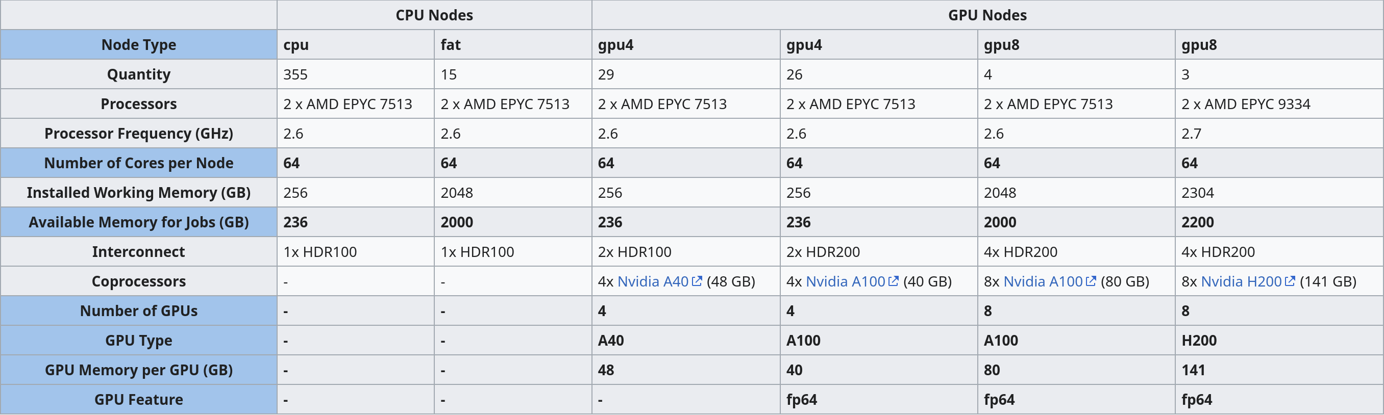
The GPU is selected by "GPU Type". The memory of each GPU Type is specified in GPU Memory per GPU (GB). For this example we select one of the A40 GPUs. Larger jobs (= longer sequences, more chains) require more memory. To access these, it is suggested to run the job directly on the Helix cluster. We will prepare a tutorial for this shortly - feel free to contact us!
You also need to define the Kernel Path to the boltz kernel at /mnt/sds-hd/sd25g005/boltz/share/jupyter/. Contact us for access to this shared directory.
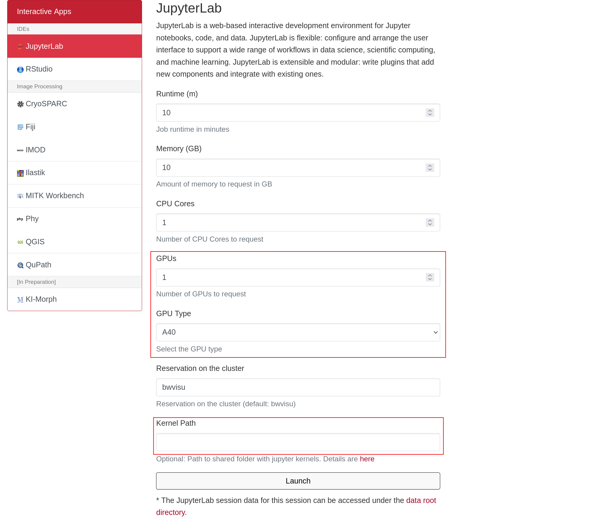
Click on "Launch". This will bring you to a new screen showing your interactive sessions. Wait for your session to be ready, then click on "Connect to Jupyter". This brings you into a JupyterLab environment.
Step 3: Set a Working Directory and Upload Files
Now we need to create and define a working directory. These will contain all files necessary for the tutorial. A new directory can be created using folder icon on the top left of the file browser:
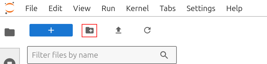
Create a working dir called boltz_test.
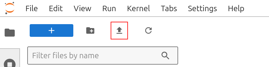
Download the tutorial notebook Boltz_w_mmseqs.ipynb from our github. Upload the notebook to bwVisu by clicking on the upload button:
You also need a .fasta file of your sequence to start. You can use our example insulin.fasta from our github
Step 4: Open the Notebook and Start the Calculation
Open Boltz_w_mmseqs.ipynb and select the boltz kernel. You can verify the kernel in the top right corner of your JupyterLab instance:

Now execute the cells in the notebook to start your Boltz run!
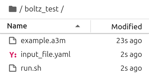
Verify Input
After running mmseqs2 and before starting your Boltz prediction you should see the following files in your working directory:
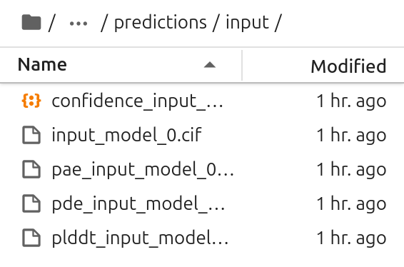
Verify Output
In the output directory, there should be multiple files. The .cif file includes the structure, the other files are used to determine the quality of the prediction.
Step 5: Analyze your results
Open the second notebook called Boltz_Confidence_Levels.ipynb to get a summary of the models confidence levels. This notebook reads the confidence descriptions and renders its central information.
To find the files, you need the name of the input file of the Boltz run and your working directory. In this example we used insulin.yaml, so the directory structure insulin is automatically created.
To visualize your predicted structures, download them to your computer and open the files with programs such as Pymol or ChimeraX. To visualize the pLDDT in "classic" AlphaFold colors, use this quick tutorial. This allows to visualize more and less confident areas of the predicted structure.
You can also further analyze the structure using the Swissmodel Structure Assessent server: https://swissmodel.expasy.org/assess
If you need more assistance with the analysis, feel free to contact us.