AlphaFold 2 on bwVisu
Welcome to the AlphaFold 2 Tutorial for bwVisu!
This tutorial will guide you through running AlphaFold 2 on bwVisu. Please follow these steps carefully. Any feedback on the tutorial is welcome! Feel free to contact us!
Preparation
Step 1: Get access to bwVisu
To start, get access to bwVisu via bwForCluster Helix or SDS. For more information, visit
https://www.urz.uni-heidelberg.de/en/service-catalogue/software-and-applications/bwvisu
For technical questions regarding the high performance cluster, see https://bw-support.scc.kit.edu. Feel free to contact us for support.
Part 1: Structure Prediction
Step 2: Connect to bwVisu and Start Jupyter
Go to https://bwvisu.bwservices.uni-heidelberg.de/ and log in with your credentials and one-time password.
Choose Jupyter and start a new session. Now you can select the resources you need.
In contrast to Alphafold 3, Alphafold 2 can run in one bwVisu job that needs both CPU and GPU resources allocated. We choose one GPU, and 16 CPU cores. We also need to account for a longer runtime, so we choose 60 minutes. If you want to execute the analysis right after the prediction, you can load the neccessary python libraries by adding /mnt/sds-hd/sd25g005/colabfold/share/jupyter to the kernel path.
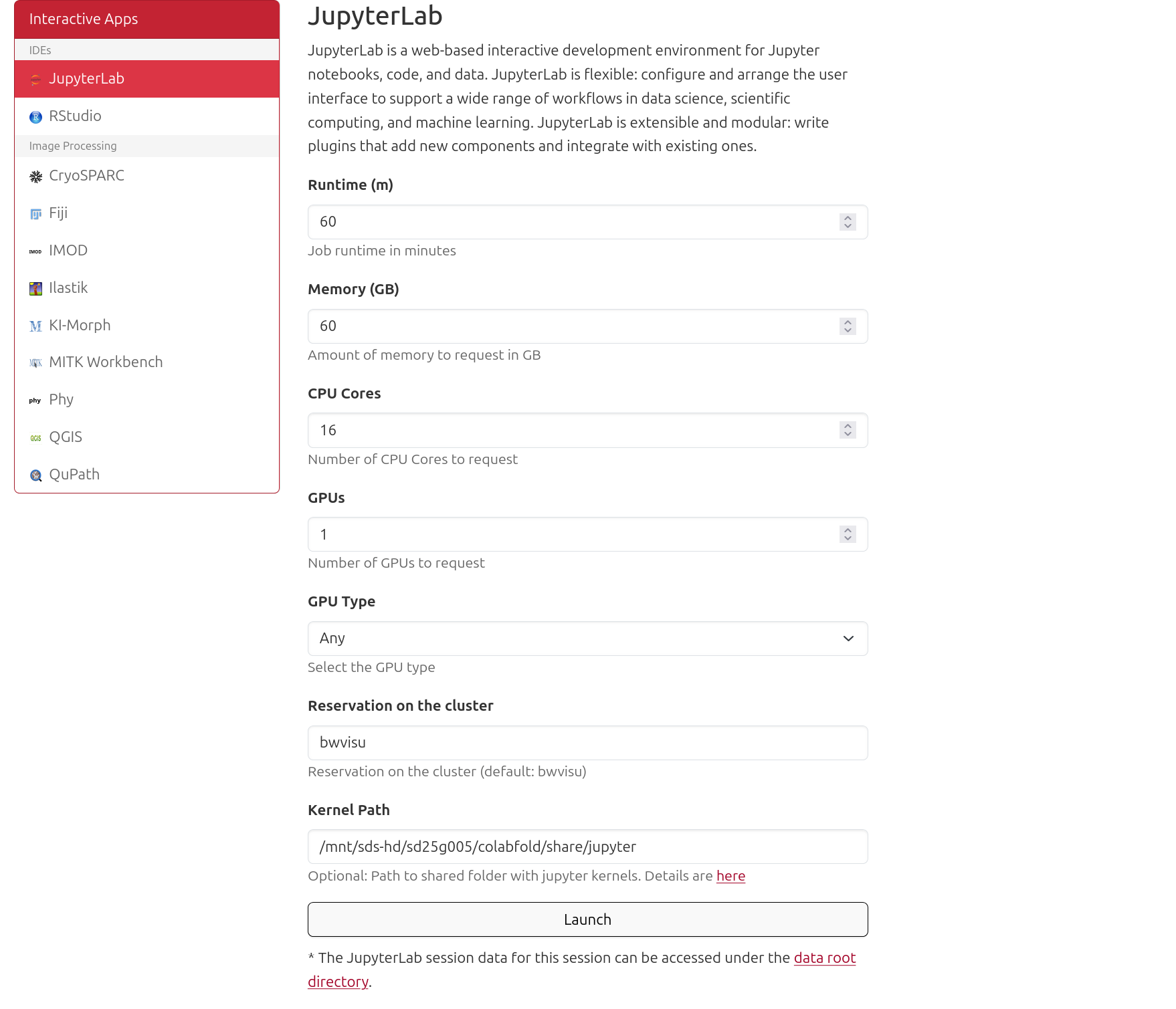
Click on "Launch". This will bring you to a new screen showing your interactive sessions. Wait for your session to be ready, then click on "Connect to Jupyter". This brings you into a JupyterLab environment.
Step 3: Set a Working Directory and Upload Files
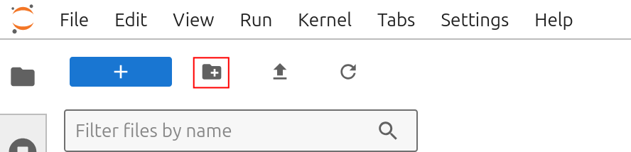
First we need to define a working directory. That can be your home or any directory you create. These will contain all files necessary for the tutorial. For this tutorial we will create a directory called alphafold2 A new directory can be created using folder icon on the top left of the file browser:
Next all required files need to be uploaded. This includes the notebooks AFold2.ipynb and AFold2_Analysis.ipynb from our github and the input sequence in .fasta format (for example, this file). You can upload these files by clicking on the upload button:
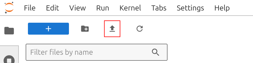
After the upload, you can see your files in the file browser on the left.
Step 4: Start the Alinment
Open Afold2.ipynb and execute the cells in the notebook to start your AlphaFold run!
Verify Input
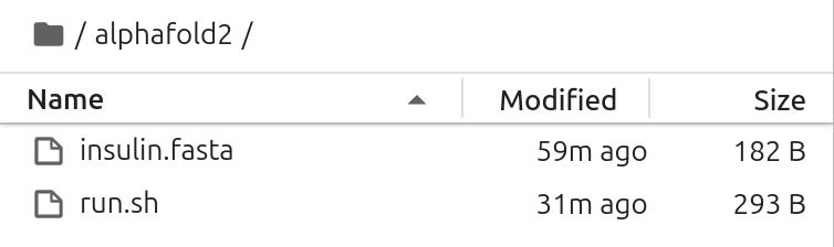
Before starting your AlphaFold 2 alignment you should see the following files in your working directory:
Verify Output
In the output directory, there should be a second directory with the same name as your .fasta file, in which you find the multi-sequence alignment (MSA), the predicted structures in .pdb file format, additional information on each structure in .pkl format, and other information in .json format.
You can find the best structure by looking at ranking_debug.json, which gives you an average ptm and iptm and the rank order. The best model will be listed at order 0. The corresponding structure is in unrelaxed_model_X_multimer_v3_pred_Y.pdb. AlphaFold 2 includes a quick MD relaxation for the best model, which you can find in relaxed_model_X_multimer_v3_pred_Y.pdb.
Part 2: Analysis
Step 5: Analyze your results
Open Afold2_Analysis.ipynb and select the colabfold kernel. You can verify the kernel in the top right corner of your JupyterLab instance.
After this, the analysis should run without any errors. Explanations of the output are provided in the notebook.
To visualize your predicted structures, download them to your computer and open the files with programs such as Pymol or ChimeraX. To visualize the pLDDT in "classic" AlphaFold colors, use this quick tutorial. This allows to visualize more and less confident areas of the predicted structure.
You can also further analyze the structure using the Swissmodel Structure Assessent server: https://swissmodel.expasy.org/assess
If you need more assistance with the analysis, feel free to contact us.